SciPy Tutorial – Learn SciPy Python Library

SciPy Tutorial for Scientific Computing in Python

SciPy is a Python library used for scientific computing, numerical analysis, optimization, statistics, signal processing, interpolation, integration, clustering, and linear algebra. It builds on NumPy arrays and provides ready-to-use algorithms for common mathematics, science, and engineering tasks.

This SciPy tutorial introduces the main SciPy modules with practical examples. You will learn how to use SciPy for k-means clustering, constants, Fourier transforms, numerical integration, interpolation, optimization, statistics, linear algebra, sparse matrices, spatial operations, and special mathematical functions.

When to Use SciPy in Python Projects

Use SciPy when a Python program needs tested numerical algorithms instead of writing mathematical routines from scratch. For example, SciPy is suitable when you need to solve equations, fit curves, compute integrals, process signals, analyze probability distributions, cluster observations, or work with matrices efficiently.

NumPy provides the array structure and many basic numerical operations. SciPy adds higher-level scientific algorithms on top of that foundation.

Install SciPy Before Running the Examples

If SciPy is not already installed, install it with pip. It is also common to install NumPy and Matplotlib because many SciPy examples use NumPy arrays and plot results.

pip install scipy numpy matplotlib

To verify the installation, import SciPy in Python and print the installed version.

import scipy

print(scipy.__version__)

Main SciPy Subpackages Covered in This Tutorial

SciPy is organized into subpackages. Each subpackage focuses on a particular area of scientific computing.

• scipy.cluster – clustering algorithms such as vector quantization and k-means
• scipy.constants – mathematical constants, physical constants, and unit conversions
• scipy.fft and scipy.fftpack – Fourier transform routines
• scipy.integrate – numerical integration and differential equation tools
• scipy.interpolate – interpolation and spline functions
• scipy.io – input and output helpers for scientific data formats
• scipy.linalg – linear algebra functions
• scipy.ndimage – multidimensional image processing
• scipy.optimize – optimization, minimization, root finding, and curve fitting
• scipy.signal – signal processing routines
• scipy.sparse – sparse matrix data structures and operations
• scipy.sparse.csgraph – graph algorithms for sparse matrices
• scipy.spatial – spatial algorithms such as distances, KD-trees, and triangulation
• scipy.stats – probability distributions and statistical functions
• scipy.odr – orthogonal distance regression
• scipy.special – special mathematical functions

SciPy Tutorial with Python Examples

The following sections explain important SciPy modules with small examples. The examples are intentionally short so that you can copy them into a Python file or a notebook and run them step by step.

SciPy Cluster Module for K-Means Clustering

Clustering is the process of organizing objects into groups whose members are similar in some way. In SciPy, clustering routines are available under scipy.cluster.

K-Means Clustering with scipy.cluster.vq

SciPy K-Means : Package scipy.cluster.vp provides kmeans() function to perform k-means on a set of observation vectors forming k clusters.

In this example, we shall generate a set of random 2-D points, centered around 3 centroids.

scipy-example.py

# import numpy
from numpy import vstack,array
from numpy.random import rand
 
# matplotlib
import matplotlib.pyplot as plt
 
# scipy
from scipy.cluster.vq import kmeans,vq,whiten
 
data = vstack(((rand(20,2)+1),(rand(20,2)+3),(rand(20,2)+4.5)))
 
plt.plot(data[:,0],data[:,1],'go')
plt.show()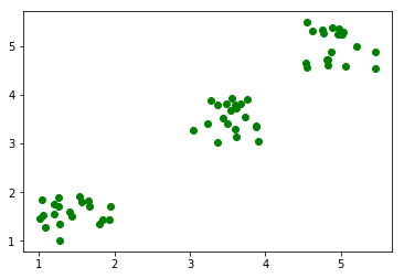

scipy-example.py

# whiten the features
data = whiten(data)

# find 3 clusters in the data
centroids,distortion = kmeans(data,3)

print('centroids  : ',centroids)
print('distortion :',distortion)
plt.plot(data[:,0],data[:,1],'go',centroids[:,0],centroids[:,1],'bs')
plt.show()

Output

centroids  :  [[ 1.42125469  1.58213817]
 [ 3.55399219  3.53655637]
 [ 4.91171555  5.02202473]]
distortion : 0.35623898893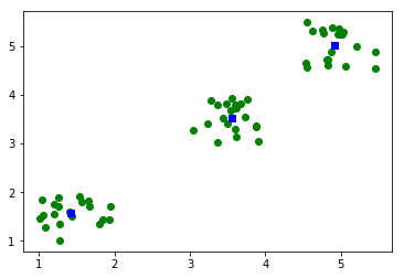

The whiten() function scales each feature by its standard deviation. This helps k-means treat both dimensions more evenly when the feature ranges are different.

After clustering, centroids contains the cluster centers and distortion gives the average distance between the observations and the nearest centroid.

SciPy Constants for Scientific Unit Values

SciPy contains physical constants, mathematical constants, and unit conversion values. These are useful when you want reliable named constants instead of hard-coding values manually.

• Mathematical Constants
• Physical Constants
• SI Prefixes(kilo, mega, zeta)
• Binary Prefixes(kibi, mebi, zebi)
• Angle: degree, arcsec, etc., in radians
• Time: minute, hour, week in seconds
• Length: mile, yard, micron, etc., in meters
• Pressure: atmosphere, torr, psi, etc., in Pascals
• Area: hectare, acre in square meters
• Volume
• Speed
• Temperature
• Energy
• Power
• Force
• Optics

The following example prints a few commonly used constants.

from scipy import constants

print(constants.pi)
print(constants.speed_of_light)
print(constants.g)
print(constants.minute)

Output

3.141592653589793
299792458.0
9.80665
60.0

SciPy FFT and FFTpack for Fourier Transforms

Fourier transform routines convert data between time or spatial domains and frequency domains. SciPy provides Fourier transform functionality through scipy.fft. Older examples may also use scipy.fftpack.

FFT with scipy.fftpack.fft

scipy.fftpack provides fft function to calculate Discrete Fourier Transform on an array.

fft-example.py

# import numpy
import numpy as np
 
# import fft
from scipy.fftpack import fft
 
# numpy array
x = np.array([1.0, 2.0, 1.0, 2.0, -1.0])
print("x            : ",x)
 
# apply fft function on array
y = fft(x)
print("fft(x)       : ",y)

Output

x : [ 1. 2. 1. 2. -1.]
fft(x) : [ 5.00000000+0.j -1.11803399-2.2653843j 1.11803399-2.71441227j
  1.11803399+2.71441227j -1.11803399+2.2653843j ]

IFFT with scipy.fftpack.ifft

scipy.fftpack provides ifft function to calculate Inverse Discrete Fourier Transform on an array.

ifft-example.py

# import numpy
import numpy as np
 
# import fft
from scipy.fftpack import fft, ifft
 
# numpy array
x = np.array([1.0, 2.0, 1.0, 2.0, -1.0])
print("x            : ",x)
 
# apply fft function on array
y = fft(x)
print("fft(x)       : ",y)
 
# ifft (y)
z = ifft(y)
print("ifft(fft(x)) : ",z)

Output

x : [ 1. 2. 1. 2. -1.]
fft(x) : [ 5.00000000+0.j -1.11803399-2.2653843j 1.11803399-2.71441227j
  1.11803399+2.71441227j -1.11803399+2.2653843j ]
ifft(fft(x)) : [ 1.+0.j 2.+0.j 1.+0.j 2.+0.j -1.+0.j]

For new code, you may prefer scipy.fft. The usage is similar for basic transforms.

import numpy as np
from scipy.fft import fft, ifft

x = np.array([1.0, 2.0, 1.0, 2.0, -1.0])
y = fft(x)
z = ifft(y)

print(y)
print(z)

SciPy Integrate Module for Numerical Integration

scipy.integrate contains functions to compute definite integrals and solve integration-related numerical problems.

In this example we will compute a definite integral using scipy.integrate.quad() function.

>>> from scipy import integrate
>>> x2 = lambda x: x**2
>>> integrate.quad(x2, 0, 4)
(21.333333333333332, 2.3684757858670003e-13)

In the first line, we imported integrate module from scipy package. Then we created a lambda function x2 which is the square of input variable. We then passed this function to the quad() function with lower limit as 0 and upper limit as 4.

In the output of quad() function, the first value is the approximate value of the integral and the second value is an estimate of absolute error.

The value is close to the exact result of the integral of x^2 from 0 to 4, which is 64/3.

SciPy Interpolate Module for Estimating Missing Values

Interpolation is the process of estimating values between known data points. It is commonly used when experimental data contains known inputs and outputs, and we need to estimate the output for new input values.

SciPy provides a variety of interpolate functions. In this example, we will take an equation y = f(x). Consider that we have performed a set of experiments and we have x values and their corresponding y values.

>>> import numpy as np
>>> from scipy import interpolate
>>> x = np.arange(0, 10)
>>> y = np.exp(-x/3.0)
>>> f = interpolate.interp1d(x, y)
>>> x
array([0, 1, 2, 3, 4, 5, 6, 7, 8, 9])
>>> y
array([1.        , 0.71653131, 0.51341712, 0.36787944, 0.26359714,
       0.1888756 , 0.13533528, 0.09697197, 0.06948345, 0.04978707])
>>> f(0.5)
array(0.85826566)
>>> f(1.5)
array(0.61497421)
>>>

interp1d() returns a lambda function and is stored in f. Now you can estimate y values for new x values. We have estimated y values for x=0.5 and x=1.5.

By default, interp1d() performs linear interpolation. You can pass the kind argument when you need a different interpolation method, such as nearest, quadratic, or cubic interpolation.

import numpy as np
from scipy.interpolate import interp1d

x = np.array([0, 1, 2, 3, 4])
y = np.array([0, 1, 4, 9, 16])

linear_function = interp1d(x, y, kind="linear")

print(linear_function(2.5))

Output

6.5

SciPy Optimize Module for Minimization and Root Finding

scipy.optimize provides functions for minimizing functions, solving equations, fitting curves, and finding roots. It is one of the most commonly used SciPy modules in data analysis and numerical computing.

The following example uses minimize() to find the value of x where a simple quadratic function has its minimum.

from scipy.optimize import minimize

def objective(x):
    return (x[0] - 3) ** 2 + 5

result = minimize(objective, x0=[0])

print(result.x)
print(result.fun)

Output

[2.99999998]
5.0

The function has its minimum near x = 3. The value of the function at that point is 5.

SciPy Stats Module for Probability Distributions

scipy.stats contains probability distributions, summary statistics, statistical tests, and random variable tools. The following example computes the probability density and cumulative distribution values for a normal distribution.

from scipy.stats import norm

print(norm.pdf(0))
print(norm.cdf(0))

Output

0.3989422804014327
0.5

Here, pdf(0) returns the value of the probability density function at zero, and cdf(0) returns the probability that a standard normal random variable is less than or equal to zero.

SciPy Linalg Module for Solving Linear Equations

scipy.linalg provides linear algebra functions such as matrix decomposition, determinants, inverses, eigenvalues, and linear system solvers. The following example solves a system of two linear equations.

Consider these equations:

3x + 2y = 12
x - y = 1

import numpy as np
from scipy.linalg import solve

A = np.array([[3, 2], [1, -1]])
b = np.array([12, 1])

solution = solve(A, b)
print(solution)

Output

[2.8 1.8]

Therefore, x = 2.8 and y = 1.8.

SciPy Sparse Module for Sparse Matrices

A sparse matrix stores mostly zero values efficiently. scipy.sparse is useful when working with large matrices in which only a small number of elements are non-zero.

import numpy as np
from scipy.sparse import csr_matrix

matrix = np.array([
    [0, 0, 3],
    [4, 0, 0],
    [0, 5, 0]
])

sparse_matrix = csr_matrix(matrix)
print(sparse_matrix)

Output

  (0, 2)	3
  (1, 0)	4
  (2, 1)	5

The output shows only the positions and values of the non-zero elements.

SciPy Spatial Module for Distance Calculations

scipy.spatial contains spatial algorithms for distance calculations, nearest-neighbor search, triangulation, and related geometry operations. The following example computes the Euclidean distance between two points.

from scipy.spatial import distance

point_a = (1, 2)
point_b = (4, 6)

print(distance.euclidean(point_a, point_b))

Output

5.0

SciPy Special Module for Mathematical Functions

scipy.special provides special mathematical functions used in scientific and engineering calculations. Examples include gamma functions, beta functions, Bessel functions, error functions, and combinatorics-related functions.

from scipy.special import gamma, comb

print(gamma(5))
print(comb(5, 2))

Output

24.0
10.0

gamma(5) returns 24 because for positive integers, gamma(n) is equal to (n - 1)!.

SciPy Module Selection Guide

Task	SciPy module to use	Common functions
Cluster observations	scipy.cluster	kmeans(), vq(), whiten()
Use scientific constants	scipy.constants	pi, speed_of_light, g
Compute Fourier transforms	scipy.fft	fft(), ifft()
Compute definite integrals	scipy.integrate	quad()
Estimate values between points	scipy.interpolate	interp1d()
Minimize functions	scipy.optimize	minimize(), root(), curve_fit()
Work with distributions	scipy.stats	norm, ttest_ind(), describe()
Solve matrix equations	scipy.linalg	solve(), inv(), eig()
Store sparse matrices	scipy.sparse	csr_matrix(), csc_matrix()

Common SciPy Errors and Practical Fixes

• ModuleNotFoundError: No module named ‘scipy’ – Install SciPy with pip install scipy in the same environment where you run Python.
• Unexpected interpolation error – Check whether the new input value lies outside the original x range. Some interpolation functions do not extrapolate by default.
• Optimization result seems wrong – Try a better initial guess, check the objective function, and inspect result.success and result.message.
• Matrix solve error – Check whether the coefficient matrix is singular or nearly singular before solving a linear system.
• Different numerical output on another machine – Small floating-point differences can happen due to library versions and numerical precision.

QA Checklist for This SciPy Tutorial

• Confirm that every SciPy code example imports the required NumPy or SciPy module before use.
• Check that output blocks are marked with the output class and not as Python code.
• Verify that examples explain the returned values, especially for quad(), kmeans(), and minimize().
• Keep older scipy.fftpack examples unchanged, but mention scipy.fft for newer Fourier transform usage.
• Review that each module section teaches a specific SciPy task instead of only listing package names.

SciPy Tutorial FAQs

What is SciPy used for in Python?

SciPy is used for scientific and numerical computing in Python. It provides algorithms for integration, interpolation, optimization, statistics, clustering, Fourier transforms, linear algebra, sparse matrices, spatial calculations, signal processing, and special mathematical functions.

What is the difference between NumPy and SciPy?

NumPy provides the core array object and basic numerical operations. SciPy builds on NumPy and provides more advanced scientific algorithms such as optimization routines, statistical distributions, integration functions, interpolation tools, sparse matrix support, and signal processing functions.

Should I use scipy.fft or scipy.fftpack?

For new SciPy code, prefer scipy.fft. Many older tutorials and examples use scipy.fftpack, and those examples may still work, but scipy.fft is the modern interface for Fourier transforms in SciPy.

Is SciPy useful for machine learning?

SciPy can be useful in machine learning workflows for optimization, clustering, statistics, distance calculations, sparse matrices, and scientific data processing. However, SciPy is a general scientific computing library, not a complete machine learning framework.

Do I need to know advanced mathematics before learning SciPy?

You can start learning SciPy with basic Python, NumPy arrays, and school-level mathematics. Some modules, such as linear algebra, optimization, signal processing, and statistics, become easier to understand when you know the related mathematical concepts.